11 min to read
Variational Autoencoders for Collaborative Filtering 리뷰
Variational Autoencoders for Collaborative Filtering
Generative 모델이란 데이터 $X$가 주어지면 그에 따른 분포로부터 새로운 샘플을 생성하는 모델입니다. 이러한 생성모델에는 여러가지 방식들이 있는데 대표적으로 설명하자면 학습 데이터의 분포를 기반으로 할 것인지(Explicit density) 혹은 그러한 분포를 몰라도 생성할 것인지(Implicit density)로 구분됩니다.
이번 포스팅에서 리뷰할 논문은 Explicit density기반의 Generative 모델인 VAE를 Neflix가 추천시스템에서 활용한 논문입니다. 모델에 대한 자세한 수식과 구조는 기존의 VAE와 크게 다르지 않습니다. 다만 어떤 분포를 가정하느냐의 차이일 뿐입니다. 이해를 위해 CS231n의 일부 슬라이드를 인용하였습니다.
ABSTRACT
논문에서 말하고자 하는 핵심은 다음과 같습니다.
- VAE를 사용함으로써 Collaborative Filtering 기반의 선형 모델들이 가지는 표현에 대한 한계점 개선.
- 다른 분야와 달리 추천시스템에서 활용되지 않았던 mulitinomial distribution기반의 generative모델을 활용하고 파라미터 추정을 위해 베이지안 추론을 사용.
- 목적함수를 학습하는데 있어서 기존 VAE의 수식과 다르게 regularization parameter를 사용하였는데anneling 기법을 통해 파라미터를 효과적으로 튜닝하여 성능을 상승.
1. INTRODUCTION
Collaborative Filtering(CF)는 유저와 아이템 간의 유사한 패턴을 찾고 이용하여 유저가 선호할 아이템들을 예측해주는 접근법입니다. CF에서는 간단하고 효율적인 Latent factor 모델들이 대부분 연구되어져왔지만 이러한 모델들은 내부적으로 선형모델이기 때문에 표현을 나타내는데 있어서 한계가 존재하게 됩니다.
또한 이전의 연구1들에서는 linear latent factor 모델에 non-linear features들을 추가함으로써 추천 성능을 크게 높일 수 있었습니다. 따라서 최근에는 신경망 기반의 CF모델의 연구들이 점점 많아지고 있습니다.
우리는 implicit feedback을 통해서 VAE가 CF를 수행할 수 있도록 확장시켰습니다. VAE는 대규모의 추천 데이터셋에서 신경망을 기반으로 linear latent factor 모델을 일반화하고 non-linear probabilistic latent-variable을 탐색합니다.
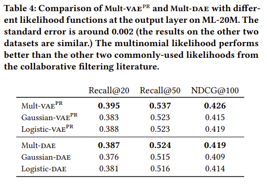
추천시스템에서는 mAP나 NDCG와 같은 랭킹 기반의 측정방식으로 평가되어지는데, TOP-N ranking loss는 최적화 되기 어려우며 direcet ranking loss는 보통 근사되어집니다. 이에 따라 우리는 multinomial likelihoods가 implicit feedback 데이터에서 잘 적합되고 Gaussian과 logistic과 같은 likelihood function보다 ranking loss를 최적화를 잘 할 수 있습니다.
추천시스템에서 거대한 수의 유저와 아이템 때문에 big-data problem으로 생각될 수 있지만 이와 대조적으로 대부분의 유저가 일부 아이템에서만 interaction이 일어난다는 점을 고려하면 small-data problem를 푸는 것과 같습니다. 이에 대해서 목표는 sparse한 signal로부터 오버피팅을 방지하고 유저의 선호도를 반영할 수 있는 probabilistic latent-variable 모델을 만드는 것입니다. 경험적으로 베이지안 접근 방식을 사용하는 것이 데이터의 sparsity에 관계없이 robust합니다.
VAE는 주로 이미지 분야에서 연구되어왔지만 추천시스템에서도 SOTA성능을 달성할 수 있었는데 그에 대한 이유로 2가지가 있습니다.
- 데이터의 분포로 multinomial likelihood를 사용
- 기존 VAE의 목적함수는 over-regularized 되었다고 해석하여 regularization term을 조정하였습니다.
2. METHOD
\[u \in\{1, \ldots, U\}\] \[i \in\{1, \ldots, I\}\] \[\mathbf{X} \in \mathbb{N}^{U \times I}\] \[\mathbf{x_u}=\left[x_{u 1}, \ldots, x_{u I}\right]^{\top} \in \mathbb{N}^{I}\]유저 $u$에 대해서 각 아이템에 대한 클릭 수를 bag-of-words 형태의 벡터로 나타낼 수 있습니다. 또한 implicit feedback문제를 다루기 위해서 click matrix는 binarize되어집니다.
2.1 Model
논문에서 고려한 generative 과정은 모든 유저 $u$에 대해서 $K$ 차원을 가지는 latent representation $z_u$에서 샘플링 되어집니다. 이 떄의 $z_u$는 prior로 Standard Gaussian분포를 가지게 됩니다.
\[\mathbf{z_u} \sim \mathcal{N}\left(0, \mathbf{I_K}\right)\]latent representation $z_u$ 는 non-linear function $f_{\theta}(\cdot) \in \mathbb{R}^{I}$ 를 통과하여 전체 $I$ 아이템에 대해서 확률 분포를 생성할 수 있습니다. non-linear function $f_{\theta}(\cdot)$ 은 파라미터 $θ$ 를 가지는 multilayer perceptron입니다. layer를 통과하고, 전체 아이템에 대한 확률 벡터 $\pi\left(\mathbf{z}_{u}\right)$를 구하기 위해서 softmax를 이용해 normalize를 수행합니다.
\[\pi\left(\mathbf{z_u}\right) \propto \exp \left\{f{\theta}\left(\mathbf{z}_{u}\right)\right\}\]$x_u$는 확률 $\pi\left(\mathbf{z}_{u}\right)$ 를 가지는 multinomial distribution분포에서 샘플링되었다고 가정합니다.
\[\mathbf{x_u} \sim \operatorname{Mult}\left(N_{u}, \pi\left(\mathbf{z}_{u}\right)\right)\]따라서 유저 $u$에 대한 log-likelihood는 아래와 같아지게 됩니다. (conditioned on the latent representation)
\[\log p_{\theta}\left(\mathbf{x_u} \mid \mathbf{z_u}\right) \stackrel{c}{=} \sum_{i} x_{u i} \log \pi_{i}\left(\mathbf{z}_{u}\right)\]click 데이터를 모델링하는데 있어서 multinomial distribution가 적합하다고 생각하였고, click matrix의 likelihood는 0이 아닌 probability mass를 가지고 있는 $x_u$ 대해서 적절한 결과를 제공합니다.
하지만 $\pi\left(\mathbf{z}_{u}\right)$ 의 합이 1이라는 제약조건이 있기 때문에 높은 선호도를 반영하는데 있어서 어느 정도 한계가 있습니다. 모델은 클릭 할 가능성이 더 높은 아이템에 더 많이 probability mass를 반영해야 합니다. 즉 가능한 추천시스템에서 평가되는 top-N ranking loss에서 잘 수행되도록 해야 합니다.
일반적으로 CF에서 latent factor에 대해 사용되는 likelihood functions(Gaussian, Logistic)과의 비교를 통해서 multinomial이 왜 더 적합한지를 추후에 설명합니다.
2.2 Variational inference
generative 모델을 학습하기 위해서는 $f_{\theta}(\cdot)$ 의 파라미터 $θ$를 추정해야 하지만 우리가 알고 싶은 posterior $p\left(\mathbf{z_u} \mid \mathbf{x_u}\right)$ 를 바로 계산할 수 없습니다.
따라서 Variational inference 기법을 이용해서 $q\left(\mathbf{z}_{u}\right)$로 $p\left(\mathbf{z_u} \mid \mathbf{x_u}\right)$를 근사합니다. 이 떄의 \(q\left(\mathbf{z}_{u}\right)\) 는 Gaussian 분포를 따른다고 가정합니다.
\[q\left(\mathbf{z_u}\right)=\mathcal{N}\left(\boldsymbol{\mu_u}, \operatorname{diag}\left\{\boldsymbol{\sigma}_{u}^{2}\right\}\right)\]따라서 Variational inference의 목적은 Kullback-Leiber divergence $\mathrm{KL}\left(q\left(\mathrm{z_u}\right) | p\left(\mathrm{z_u} \mid \mathrm{x}_{u}\right)\right)$ 를 최소화시킴으로써 \(\left\{\boldsymbol{\mu}_{u}, \boldsymbol{\sigma}_{u}^{2}\right\}\)를 추정하는 것입니다.
2.2.1 Amortized inference and the variational autoencoder
데이터셋에서 유저와 아이템의 수가 커질수록 optimize를 해야하는 \(\left\{\boldsymbol{\mu}_{\boldsymbol{u}}, \boldsymbol{\sigma}_{\boldsymbol{u}}^{2}\right\}\) 의 파라미터 수도 점점 많아지게 됩니다. 즉 이는 수백만명의 유저와 아이템이 있는 추천시스템에서는 병목 현상(bottleneck)이 발생할 수 있습니다. 따라서 VAE에서는 data-dependent한 함수를 통하여 파라미터가 추정되도록 합니다.
\[g_{\phi}\left(\mathbf{x_u}\right) \equiv\left[\mu_{\phi}\left(\mathbf{x_u}\right), \sigma_{\phi}\left(\mathbf{x}_{u}\right)\right] \in \mathbb{R}^{2 K}\]좀 더 추가적인 설명을 덧붙이자면 이는 $\mathbf{z}$에 대한 사전 분포 prior를 가정하였기 때문에 MLE를 통해서 바로 $\mathbf{x}$를 추정할 수 있지만 prior에서 sampling 하는 것은 데이터가 많아질수록 병목현상이 있다고 하는 것입니다. 따라서 $\mathbf{x}$와 유의미하게 $\mathbf{z}$가 나올 수 있도록 sampling을 합니다.
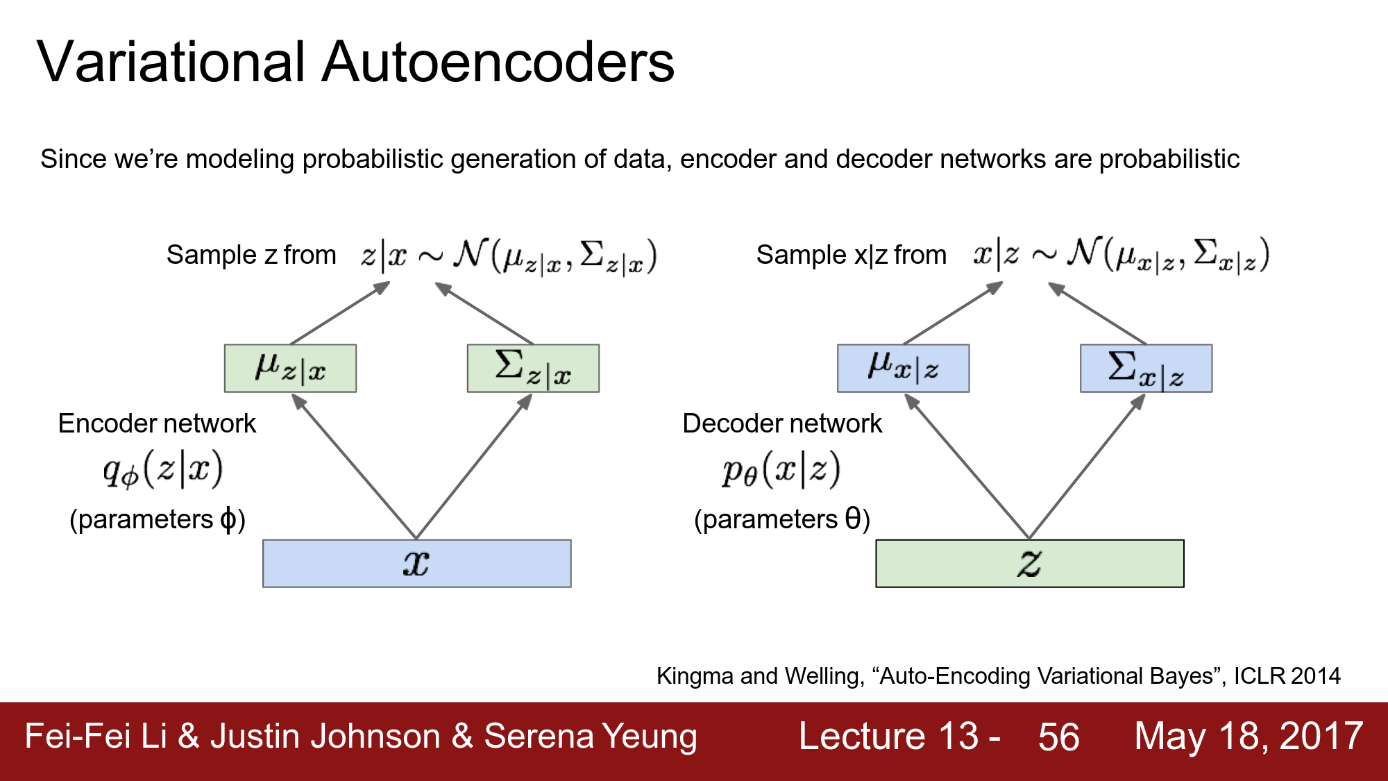
\(\mu_{\phi}\left(\mathbf{x}_{\mathbf{u}}\right)\) 와 \(\sigma_{\phi}\left(\mathbf{x}_{u}\right)\) 는 모두 $\phi$에 대한 파라미터가 되며, 이에 따라 posterior에 근사하는 분포 variational distribution를 만들어 낼 수 있습니다.
\[q_{\phi}\left(\mathbf{z_u} \mid \mathbf{x_u}\right)=\mathcal{N}\left(\mu_{\phi}\left(\mathbf{x_u}\right), \operatorname{diag}\left\{\sigma_{\phi}^{2}\left(\mathbf{x}_{u}\right)\right\}\right)\]요약하면 관찰된 데이터 $\mathbf{x_u}$를 input으로 사용하여, posterior에 근사하는 분포 variational distribution $q_{\phi}\left(\mathbf{z_u} \mid \mathbf{x_u}\right)$ 를 통하여 variational parameters를 추정합니다.
$q_{\phi}\left(\mathbf{z_u} \mid \mathbf{x_u}\right)$ 와 generative model $p_{\theta}\left(\mathbf{x_u} \mid \mathbf{z_u}\right)$ 을 통해서 샘플링을 하는데 이 구조가 autoencoder구조를 가진다고 하여 variational autoencoder라 부릅니다.
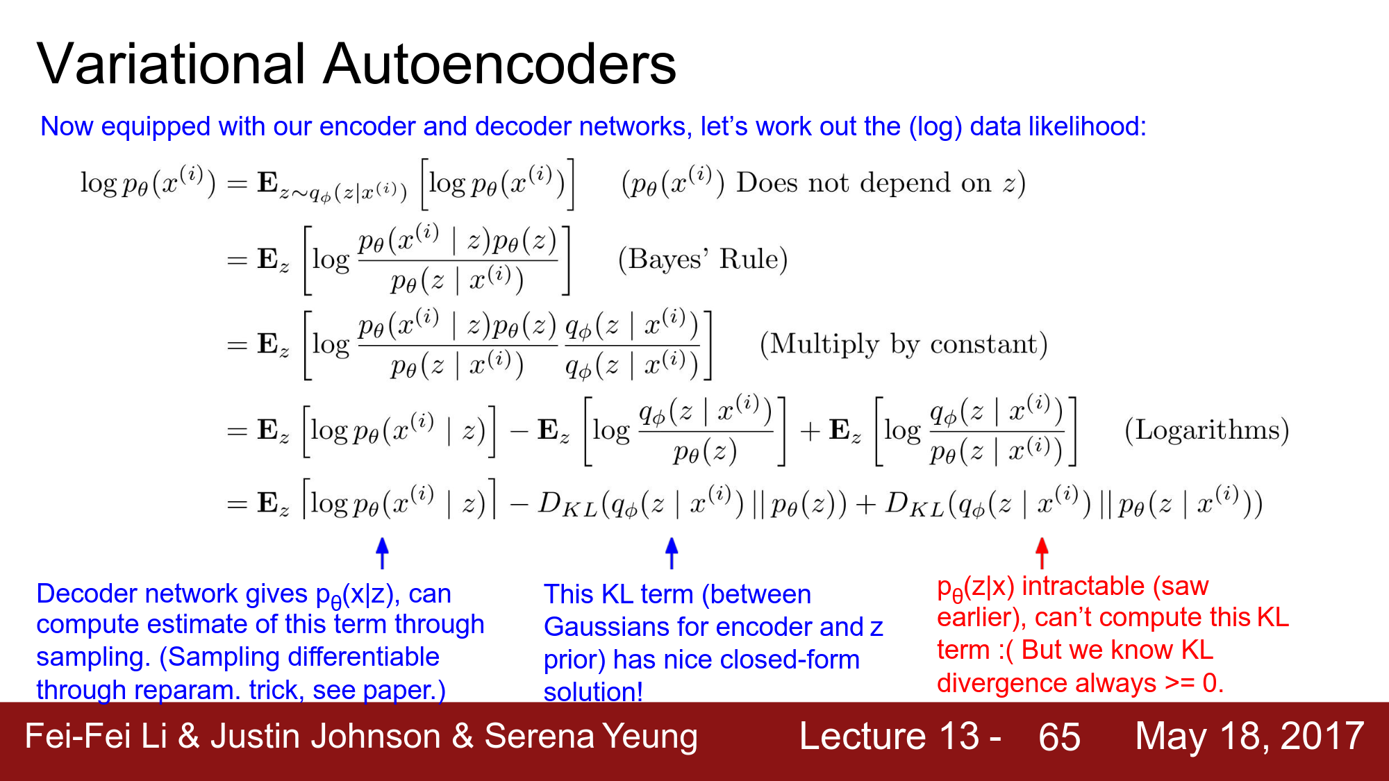
VAE는 marginal likelihood를 통하여 lower bound를 최대화하고자 합니다.
\[\begin{aligned} \log p\left(\mathbf{x_u} ; \theta\right) & \geq \mathbb{E}_{q_{\phi}\left(\mathbf{z_u} \mid \mathbf{x_u}\right)}\left[\log p_{\theta}\left(\mathbf{x_u} \mid \mathbf{z_u}\right)\right]-\mathrm{KL}\left(q_{\phi}\left(\mathbf{z_u} \mid \mathbf{x_u}\right) \| p\left(\mathbf{z_u}\right)\right) \\ & \equiv \mathcal{L}\left(\mathbf{x_u} ; \theta, \phi\right) \end{aligned}\]$p(x)$ 는 베이즈 정리에서 evidence라고 이름이 붙여진 항이기 때문에 위의 부등식의 우변을 Evidence Lower Bound(ELBO)로 알려져 있습니다. ELBO는 $\theta$ 와 $\phi$ 를 가지는 함수로 stochastic gradient ascent를 통하여 파라미터를 추정합니다. 하지만 $\mathbf{z_u} \sim q_{\phi}$ 와 같은 sampling 과정이 포함되어 있기 때문에 gradinet를 얻는 것이 어려워 reparametrization trick을 사용하여 해결합니다.
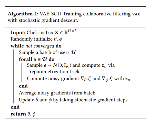
\(\boldsymbol{\epsilon} \sim \mathcal{N}\left(0, \mathbf{I}_{K}\right)\) 에서 샘플링하여 \(\mathbf{z_u}=\mu_{\phi}\left(\mathbf{x_u}\right)+\boldsymbol{\epsilon} \odot \sigma_{\phi}\left(\mathbf{x}_{u}\right)\) 로 다시 reparameterize시킵니다.
샘플링 과정이 isolated 되어 샘플링 되어진 $\mathbf{z_u}$를 통해 back-propagated가 가능하게 되어 $\phi$에 대한 gradient를 얻을 수 있습니다. 수식의 유도 과정은 아래의 슬라이드를 참고 바랍니다.
위에 대한 모든 과정은 아래 Algorithm 1에 설명되어 있습니다.
2.2.2 Alternative interpretation of elbo
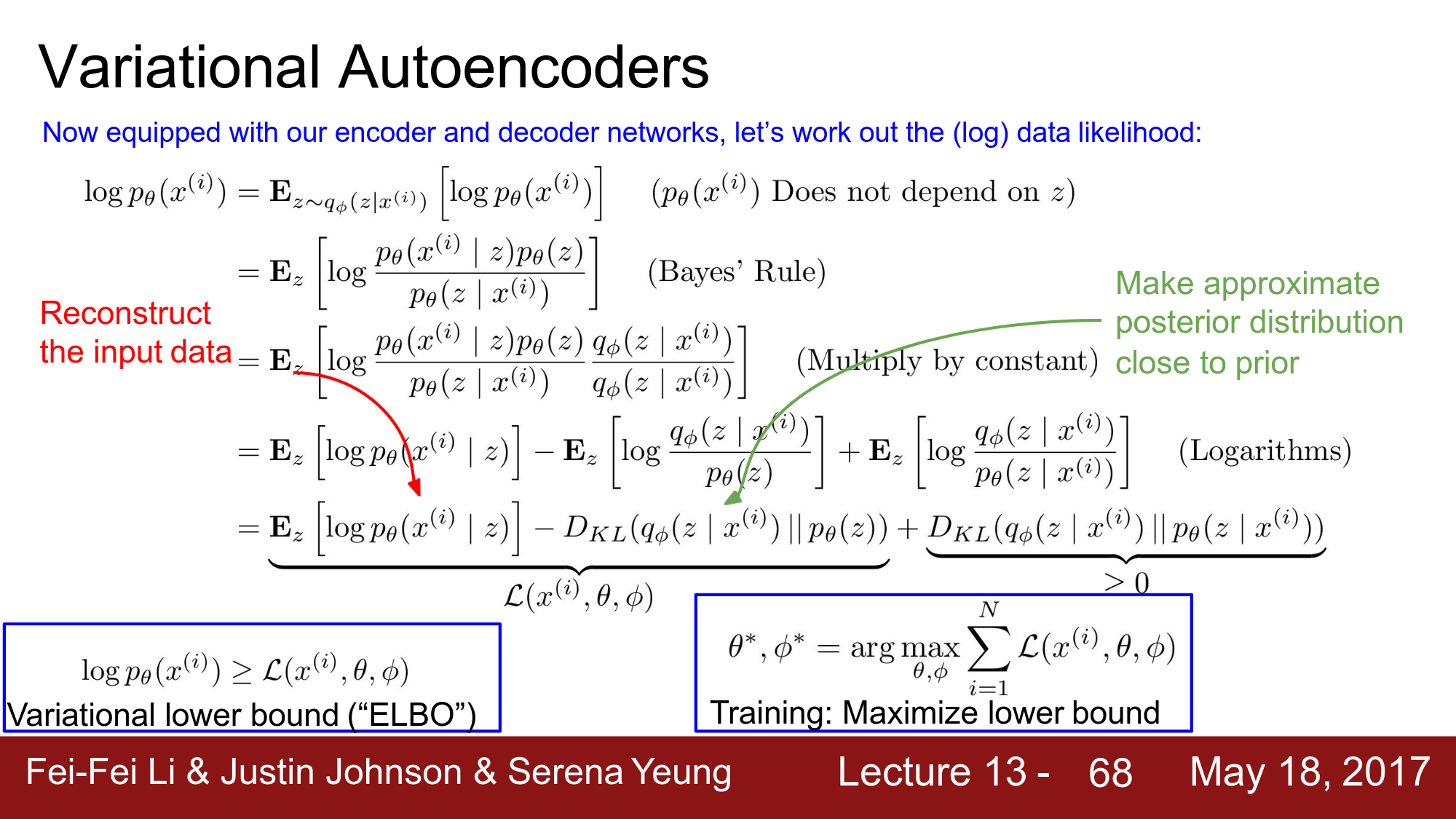
위에서 정의한 ELBO의 수식을 통해 가능도 함수를 구하여 loss를 최소화 하는 것이 목적이므로 수식에 -를 곱하게 된다면 \(\mathbb-{E}_{q_{\phi}\left(\mathbf{z}_{u} \mid \mathbf{x}_{u}\right)}\left[\log p_{\theta}\left(\mathbf{x_u} \mid \mathbf{z_u}\right)\right]+\mathrm{KL}\left(q_{\phi}\left(\mathbf{z_u} \mid \mathbf{x_u}\right) \| p\left(\mathbf{z_u}\right)\right)\) 가 됩니다.
첫번쨰 항은 샘플링 함수에 대한 negative log likelihood인 reconstruction error이고 posterior와 prior를 유사하도록 만드는 KL term은 regularization으로 볼 수 있습니다. 이는 trade-off 관계이며, 논문에서는 이러한 regularization를 조절할 수 있는 파라미터 $\beta$를 도입함으로써 ELBO를 확장시켰습니다.
\[\mathcal{L}_{\beta}\left(\mathbf{x}_{u} ; \theta, \phi\right) \equiv \mathbb{E}_{q_{\phi}\left(\mathbf{z}_{u} \mid \mathbf{x}_{u}\right)}\left[\log p_{\theta}\left(\mathbf{x_u} \mid \mathbf{z_u}\right)\right]-\beta*\mathrm{KL}\left(q_{\phi}\left(\mathbf{z_u} \mid \mathbf{x_u}\right) \| p\left(\mathbf{z_u}\right)\right)\]파라미터 $\beta$를 선택하는 과정은 heuristic하게 0부터 시작하여 1까지 점진적으로 증가시키면서 $\beta$를 탐색하였으며, 이러한 탐색과정을 KL annealing이라 합니다.
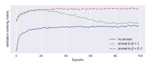
- KL annealing 과정 수행의 유무는 성능 차이에 큰 영향이 있었습니다 (Blue)
- $\beta$를 1까지 annealing하게 된다면 1에 가까워 질수록 성능이 떨어집니다 (Green)
- 따라서 peak지점까지 다시 $\beta$를 annealing 하였을 떄, 가장 성능이 우수하였습니다 (Red)
- 이러한 annealing 과정은 VAE를 학습하는데 있어서 추가적인 runtime를 초래하지 않습니다.
이와 같이 multinomial likelihood기반의 partially regularized 되어진 VAE를 $\text { Mult-VAE }^{\mathrm{PR}}$ 라 합니다. 포스팅에서는 Mult-VAE 로 쓰겠습니다.
2.2.3 Computational Burden
지금까지의 neural network기반의 CF 모델들은 click matrix로부터 (user, item)으로 구성된 single entry를 받아서 파라미터를 업데이트하였지만 Algorithm 1과 같이 VAE에서는 user를 subsample하여 user의 전체 click history를 이용하여 모델 파라미터를 업데이트 합니다. negative examples의 수를 정하여 negative sampling를 수행하는 hyperparameter tuning의 과정이 필요하지 않기 때문에 계산적 측면에서 유리합니다.
그러나 아이템의 수가 워낙 크기 때문에 multinomial probability $\pi\left(\mathbf{z}_{u}\right)$ 를 계산하는데 어려움이 있습니다. 실험결과로 50K개의 아이템보다 적은 medium-to-large 사이즈의 데이터에서는 computational bottleneck이 나타나지 않았지만 아이템이 더 많아질 수록 bottleneck이 발생할것입니다.
따라서 $\pi\left(\mathbf{z}_{u}\right)$에 대해 normalization factor로 근사하는 기법을 제안한 논문2에서의 방법을 적용할 수 있습니다.
2.3 A taxonomy of autoencoders
autoencoder관점에서 연구를 수행하였는데 먼저 AE에 대한 Maximum-likelihood는 아래와 같습니다.
\[\begin{aligned} \theta^{\mathrm{AE}}, \phi^{\mathrm{AE}} &=\underset{\theta, \phi}{\arg \max } \sum_{u} \mathbb{E}_{\delta\left(\mathbf{z}{u}-g_{\phi}\left(\mathbf{x}{u}\right)\right)}\left[\log p_{\theta}\left(\mathbf{x}_{u} \mid \mathbf{z}_{u}\right)\right] \\ &=\underset{\theta, \phi}{\arg \max } \sum_{u} \log {p}_ \theta\left(\mathbf{x}_{u} \mid g_{\phi}\left(\mathbf{x}_{u}\right)\right) \end{aligned}\]AE와 DAE는 지금까지의 VAE와는 구분되는 특징이 있습니다.
- VAE에서 prior를 근사하는 variational distribution $q_{\phi}\left(\mathbf{z_u} \mid \mathbf{x_u}\right)$를 regularize하지 않습니다. 즉 \(q_{\phi}\left(\mathbf{z}_{u} \mid \mathbf{x}_{u}\right)=\delta\left(\mathbf{z}_{u}-g_{\phi}\left(\mathbf{x}_{u}\right)\right)\) 를 통해서 optimize 됩니다.
실제로 AE를 학습할 때, $\mathbf{x}_{u}$ 중 non-zero인 entry에 대해서 모든 probability mass를 계산하기 때문에 쉅게 overfitting 되어집니다. DAE에서는 input layer마다 dropout를 적용함으로써 overfitting을 방지하고 성능을 개선시켰습니다.
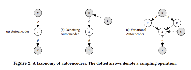
따라서 Mult-VAE와 함께 multinomial likelihood 기반의 denoising autoencoder도 Mult-DAE 같이 연구하였습니다.
2.4 Prediction
훈련된 generative model을 통해서 어떻게 예측이 이루어지는지 살펴봅니다.
Mult-VAE와 Mult-DAE 모두 같은 방식으로 예측을 하며 유저의 click history $\mathbf x$가 주어지면 un-normalized된 multinomial probability $f_θ(z)$를 통하여 모든 아이템에 rank를 매깁니다. $\mathbf x$에 대한 latent representation $\mathbf z$는 모델에 따라서 아래와 같이 구성됩니다.
Mult-VAEvariational distribution의 평균, $\mathbf{z}=\mu_{\phi}(\mathbf{x})$Mult-DAE$\mathbf{z}=g_{\phi}(x)$
결국 $\mathbf z$를 분포로 나타내기 위해 평균을 사용할지 하나의 single value로 나타낼지의 차이로 볼 수 있습니다.
3 RELATED WORK
-
Vaes on sparse data
최근 연구3들에 의하면 VAE는 large, sparse, high-dimensional한 데이터를 모델링 할 때 underfitting 된다고 알려져있습니다. 논문에서도 annealing을 수행하지 않거나 $\beta = 1$로 설정할 경우, 비슷한 이슈가 있었습니다. 따라서 ancestral sampling을 수행하지 않고 $\beta \leq 1$ 로 설정하게 되면 적절한 generative model이 아닐수도 있지만 collaborative filtering 관점에서 항상 유저의 click history에 기반하여 예측합니다.
-
Information-theoretic connection with VAE
위에서 정의한 ELBO의 regularization term은 Bayesian inference와 generative modeling을 통해서 Maximum-entropy discrimination을 수행하며, $\beta$는 모델의 discriminative와 generative의 부분을 조절하는 역할을 하게 됩니다. 다시 말하면 유저의 click history를 기반으로 최대 엔트로피를 가지는 분포를 찾는 것이며, 이 떄 $\beta$를 통해 prior를 얼마나 반영할지를 조절할지를 결정하는 파라미터라고 볼 수 있습니다.
-
Neural networks for collaborative filtering
초기 neural network기반의 CF모델들은 explicit feedback의 데이터와 rating을 예측하는 것에 집중하였지만 최근에는 implicit feedback의 중요성이 높아져가면서 그에 대한 연구들이 진행되어졌습니다. 이에 대해 우리의 연구와 관련된 중요한 논문들은 collaborative denoising autoencoder와 neural collaborative filtering입니다.
CDAE와NCF모두 유저와 아이템의 수에 따라서 모델의 파라미터가 점진적으로 증가하기 떄문에 이는 larger datasets에서는 문제가 될 수 있음을 파악하고 각 데이터셋에 대해 실험하였습니다.
4 EMPIRICAL STUDY
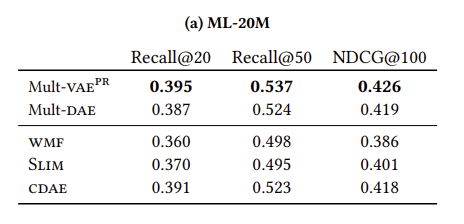
Mult-VAE 와 Mult-DAE 두 모델에 대한 성능을 측정하였고, 실험에 따른 주요 결과는 아래와 같습니다.
Mult-VAE은 최근에 제안된 neural-network-based CF 모델들보다 SOTA성능을 달성하였습니다.- DAE와 VAE에서 multinomial likelihood를 사용하는 것이 다른 Gaussian이나 logistic likelihoods보다 좀 더 유리하였습니다.
Mult-VAE와Mult-DAE를 비교하였을떄, 항상 특정 모델의 성능이 높게 나오지는 않기 때문에 두 모델에 대한 접근법의 장단점을 정리하였습니다.
4.1 Datasets
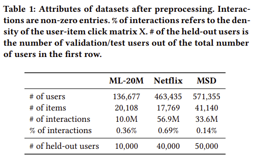
다양한 도메인에서 3개의 medium-to large 사이즈의 user-item consumption 데이터를 기반으로 실험하였습니다.
- MovieLens-20M (ML-20M)
- Netflix Prize (Netflix)
- Million Song Dataset (MSD)
Table1에 모든 데이터셋에 대한 전처리 후의 결과를 요약하였습니다.
4.2 Metrics
Recall@R, NDCG@R 두 개의 rank metric을 사용해 성능을 평가하였습니다. 각 유저에 대해서 held-out 아이템에 대한 predicted rank와 true rank를 비교합니다.
$\omega(r)$ 은 아이템에 대한 rank $r$ 이며, $\mathbb{I}[\cdot]$ 는 indicator function, $I_{u}$ 는 유저가 click한 held-out 아이템들의 집합을 뜻하며, 아래와 같이 정의됩니다.
\[\text {Recall@R }(u, \omega):=\frac{\sum_{r=1}^{R} \mathbb{I}\left[\omega(r) \in I_{u}\right]}{\min \left(M,\left|I_{u}\right|\right)}\] \[\operatorname{DCG} @ R(u, \omega):=\sum_{r=1}^{R} \frac{2^{\mathbb{I}\left[\omega(r) \in I_{u}\right]}-1}{\log (r+1)}\]NDCG@R은 위의 DCG@R을 0에서 1사이로 normalize를 수행한 metric입니다.
4.3 Experimental setup
strong generalization를 위해서 모든 유저들을 training / validation / test sets으로 split하였습니다.
training users들의 전체 click history를 기반으로 모델을 학습하며, held-out (validation and test)의 경우, user들의 전체 click history가 아니라 모델이 필요한 user-level representation을 학습하기 위한 click history의 일부분만을 이용하여 평가합니다.
즉 held-out user들의 unseen한 click history 에서도 모델이 얼마나 rank를 잘 평가할 수 있는지를 평가하기 위함입니다.
generalization보다 상대적으로 더 어려운 것은 training과 evaluation에서 모두 user’s click history가 나타날 경우 어떻게 처리하는지의 문제입니다.
이를 해결하기 위해서 각 held-out user들의 click history에서 80%를 랜덤하게 선택하여 fold-in set을 구성하여 모델이 user-level representation를 학습하게 하고 나머지 20%의 click history에 대해서 평가하였습니다.
validation users에 대한 NDCG@100를 기반으로 모델의 hyperparameter와 architectures를 선택하였습니다. Mult-VAE와 Mult-DAE 의 전반적인 모델 구조는 1-hidden-layer를 가지는 MLP generative model이며 실험적으로도 0~1개의 hidden layer의 구조가 성능이 우수하였습니다.
Same
- input layer에 대해서 dropout(p=0.5)를 적용
- batch_size= 500
- opimizer = Adam
- ML-20M 데이터셋의 경우, 200 epoch 동안 train
Difference
Mult-DAE의 경우 input layer에 대해서 tanh activation function을 적용하고 weight decay 수행Mult-VAE는 encoder의 output이 gaussian 분포로 사용되기 때문에 0-hidden-layer MLP 구조가 사용되었음
4.4 Baselines
- Weighted matrix factorization (WMF)
- SLIM
- Collaborative denoising autoencoder(CDAE)
- Neural collaborative filtering(NCF)
- Bayesian personalized ranking(BPR)의 경우 다른 baseline 모델보다 성능이 너무 낮아서 포함시키지 않음
4.5 Experimental results and analysis
-
Quantitative results
-
How well does multinomial likelihood perform?
-
When does
Mult-VAEperform better/worse thanMult-DAE?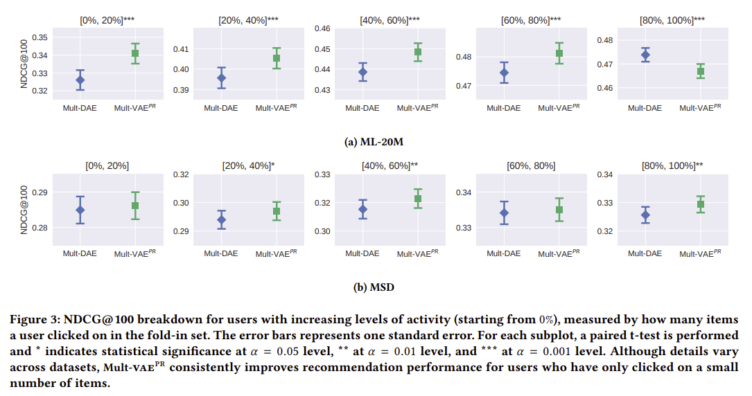
Reference
-
Dawen Liang, Jaan Altosaar, Laurent Charlin, and David M. Blei. 2016. Factorization meets the item embedding: Regularizing matrix factorization with item co-occurrence. In Proceedings of the 10th ACM conference on recommender systems. 59–66 ↩
-
Aleksandar Botev, Bowen Zheng, and David Barber. 2017. Complementary Sum Sampling for Likelihood Approximation in Large Scale Classification. In Proceedings of the 20th International Conference on Artificial Intelligence and Statistics. 1030–1038 ↩
-
Rahul G. Krishnan, Dawen Liang, and Matthew D. Hoffman. 2017. On the challenges of learning with inference networks on sparse, high-dimensional data. arXiv preprint arXiv:1710.06085 (2017). ↩
Comments